


developer_ah
-
Posts
28 -
Joined
-
Last visited
-
Days Won
5
Everything posted by developer_ah
-
The topics of the webinar: - On-Grid system - with net metering and electric vehicle - MeteoSyn - Load profiles - Photo Plan, Roof view - Polymorphic configuration and power optimizers
-
- 2
-

-
- power optimizers
- polymorphic configuration
- (and 7 more)
-
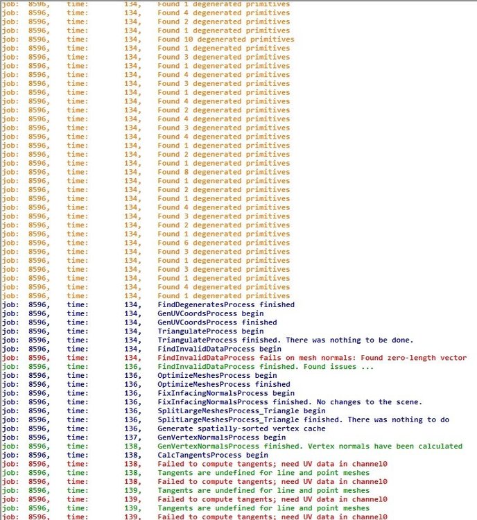
Hallo Alex, ich habe ebenfalls die .3ds-Files heruntergeladen und ausprobiert und ja, keines der Files lässt sich in PV*SOL laden. Um solche Dateien laden zu können, benutzt PV*SOL intern einen Importer, der erst das .3ds-File in ein .obj-File umwandelt. Normalerweise funktioniert das auch. Ich habe gerade geprüft, ob andere .3ds-Dateien noch geladen werden können. Keine Probleme. Also habe ich Open3Mod geöffnet. Das ist ein kostenloses Tool, mit dem man 3D-Dateien anschauen und auch in andere Formate konvertieren kann. Das kannst du gern mal ausprobieren. Dieses Tool nutzt dieselbe Schnittstelle, wie wir, repariert aber noch mehr degenerierte Files, als PV*SOL es kann. Das Tool hat ein Logfile angelegt (Screenshot habe ich beigefügt). Dieses Logfile zeigt jede Menge Unstimmigkeiten bei den Files an. Es ist mir nicht einmal gelungen, es selbst in .obj umzuwandeln. Daher schlage ich vor, du nimmst die Files, die auf der Homepage in anderen Formaten vorliegen und versuchst sie mit Blender oder andere freien Konverter (z.B. Open3Mod) erst einmal in ein komplett fehlerfreies .obj-File umzuwandeln und erst dann in PV*SOL zu laden. Viele Grüße, Chris
-
Extract Google Earth 3D models with Pix4D and PV*SOL
developer_ah replied to Low Carbon Exchange's topic in PV*SOL
You're alluding to a tutorial that one of our partners did. Unfortunately, we cannot present external software programs in the PV*SOL Forum. I can only say that I personally use the c't tool ac'tivAid to make screenshots. In addition, these should be done in the best possible resolution for the monitor and also at least 30 from different angles! -
Extract Google Earth 3D models with Pix4D and PV*SOL premium 2018 http://www.valentin-software.com/services/fw/yt-tut-en/dl-pvsolprem-en [Full Traskript] 1. Create screenshots in Google Earth Pro 2. Photogrammetry with Pix4D 3. Import of the 3D model into PV*SOL premium First, start Google Earth Pro. For this video I chose a free-standing, relatively complex building in England. Here I enter the coordinates of the object. A 3D model is to be extracted from this object. First, I determine the size of an edge of the model. This is later used in PV*SOL to reproduce the scale. To do this I use the ruler function of Google Earth and draw a 3D path to an edge that is well visible. The measured length of the edge is approx. 20m. In the next step I will take about 30 - 40 screenshots of the scene to create a 3D model in Pix4D. In order to achieve an optimal result with photogrammetry, all labels and menus should be hidden first. Now the screenshots can be made. Recommendation: take pictures at 3 different altitudes: - 12 pictures at the height of the ridge or the highest point of the building. - 8 pictures from different angles of the bird's eye view - 12 pictures at a height of 3 meters Make sure - that the target building is always completely visible, - that potential additional shading objects are visible, - and that the pictures are not too twisted. The more images that are created from different perspectives, the better the 3D model created later on will be. In some photogrammetry programs it is useful to take some close-ups as well. Also move the mouse out of the picture before creating the screenshot, so that the mouse cursor is not visible in the picture! After you have made the 30-40 screenshots, start Pix4Desktop. You can currently download this program as a 14-day trial version by creating a customer account on: https://pix4d.com/product/pix4dmapper-photogrammetry-software/ After you have started Pix4Dmapper Pro, you will be taken to the "Home" page of the program. First, create a new project. The "New Project"dialog opens. Here you can select the project folder. Enter the project name here. In the next step the screenshots will be added. Click on "Add Images". Now select all screenshots with "Ctrl-A". The following message can be ignored. Here you can now see an overview of the geodata and the camera model, which were determined from the images. Due to the fact that I made screenshots, not much data is included. The following pages are currently not interesting. Click your way through. On the last page you can see an overview of the level of detail expected for the finished 3D model and how long the creation process will probably take. Select the menu item "3D Models" and then click "Finish". The map view is now displayed. This is not interesting at the moment, because there is no geoinformation in the pictures. The next step is to create the 3D model. Before I click on "Start", let's first look at the options for this. Click "Process", and then click "Process Options". At first, only the settings for "Process" and "Point Cloud and Mesh"are interesting. I leave the general process options unchanged. Make sure that "Keypoints Image Scale" --> "Full" is selected. You can experiment a little later on with the settings for the "Point Cloud" to get an even better result. I leave the settings unchanged. A few things have to be adapted to the mesh options so that the 3D model can be imported correctly into PV*SOL premium later on. I want the textures from the screenshots to be transferred into the 3D model. We set the "Maximum Octree Depth" to 14. The maximum "Texture Size" should be 4096 pixels. The maximum number of triangles has to be limited for the level of detail, because PV*SOL premium currently only accepts 3D models with a maximum of 500,000 points. You can achieve this with the decimation strategy "Sensitive". A model file is automatically generated after photogrammetry is complete. Here you specify that this file is to be created in obj format. Now the 3D model can be created. First, perform step 1 only! This process can take several minutes. I'm fast-forwarding. The result now shows the reproduced positions of the camera and the tie points. The camera positions can be hidden. Unfortunately, the program sometimes has difficulties in determining the correct position of the model from the screenshots. Here you can see a completely unnatural slope which has to be corrected. The "Orientation Constraints" function is used to correct the alignment and inclination of the model. Place the ends of the 3D arrow at a distance you know to be parallel to the height axis. (Here z-axis!!) Step 1 must now be revised. The model has now been corrected. Next, the triangle mesh can be generated. I'm fast-forwarding again. Now the 3D model is already complete and can be viewed. If you want to view the mesh, you must first activate "Triangle Meshes". I just want to view the triangulated mesh and disable the other elements. You can see that the 3D model is already close to the Google original. Now open PV*SOL premium 2018 or a higher version! I am already in the 3D visualization of PV*SOL premium and have started a new project there. Now import the 3D model you created with Pix4D. To do so, click this button. You will find the. obj file, as well as materials and texture in the project folder that Pix4D has created. I simply place the 3D model in the middle of the terrain. As you can see, the 3D model is stored in an unusual coordinate system, which has to be corrected. To do this, double-click on the model and select the "Tilt backward" option. The model has also been well imported into PV*SOL premium. Here already with representation of the shading. Now check the distance measured in Google Earth. To do this, draw a PV area polygon. As you can see, the model is not to scale. It must be corrected (see video). The alignment must also be adjusted! The building can then be covered with PV modules. End of the tutorial. Thank you for watching! The computer program shown is PV*SOL premium, a design software by Valentin Software in the field of photovoltaics / renewable energy. The priorities of this software are design support and yield calculation. The integrated 3D visualization determines the impact of shading on the yield. Another focus is on the cost-effectiveness of photovoltaic systems with and without self-consumption
-
Hello James, could you please contact our support and, if necessary, also send the projects mentioned? I'll look into it then. Thank you very much. hotline@valentin-software.com Many greetings.
-
Hello Stuart, yes, 400MB ist far to much. PV*SOL ist a 32 Bit application. So the maximum size ist 250MB and the maximum number of points is 500.000. But even this can be to much, if you want to do a fast planning. Make you life as easy as possible and reduce the files on a minimum. The greather a model file, the more time PV*SOL need to calculate for ex. the shading, because every single Triangle of the model now can evoke shading. We apoligize the empty message. Its a error. It says that the file ist too big. Many greetings!
-
Hallo, ja, das ist ja schon eine nette Idee, die Sperrabstände in den Default-XMLs zu ändern. Bei den Randabständen ist das nicht so einfach, weil nur die Randabstände, welche geändert wurden, in einer Projekt-XML im Tempordner abgelegt werden. Diese nachträglich zu ändern, macht keinen Sinn, weil die Datei bei jedem neuen Projekt neu angelegt wird. Eine Möglichkeit wäre, sich ein Rumpfprojekt anzulegen mit einem Gebäude, welches überall die gewünschten Randabstände hat. Das gleiche gilt für das Montagesystem für die Modulaufständerung. Einfach anlegen und mit dem Rumpfprojekt abspeichern. Man könnte sich sogar ein paar vorgefertigte Fenster und andere 3D-Objekte auf einem anderen Gebäude anlegen und diese bei der Planung auf das Gebäude kopieren. Das "Als Standard speichern" beim Montagesystem funktioniert derzeit leider nur innerhalb eines Projekts. Die Werte sollten natürlich auch bei "Projekt Neu" zur Verfügung stehen. Wir werden das aufnehmen. Den Standort als "Standard" speichern, funktioniert bei mir. Nach Projekt Neu wird immer der neue Standort angezeigt. Viele Grüße
-
http://www.valentin-software.com/services/fw/yt-tut-de/dl-pvsolprem-de 1. Screenshots anfertigen in Google Earth Pro 2. Photogrammetrie mit Pix4D 3. Import des 3D-Modells in PV*SOL premium Starten Sie zunächst Google Earth Pro. Für dieses Video habe ich ein frei stehendes, relativ komplexes Gebäude in England gewählt. Ich gebe hier nun die Koordinaten des Objekts ein. Von diesem Objekt soll ein 3D-Modell extrahiert werden. Als Erstes ermittle ich die Abmessung einer Kante des Modells. Diese wird später in PV*SOL benötigt, um den Maßstab zu reproduzieren. Hierzu nutze ich die Lineal-Funktion von Google Earth und zeichne einen 3D-Pfad an eine gut sichtbare Kante. Die gemessene Länge der Kante beträgt ca. 20m. Im nächsten Schritt werde ich von der Szene ca. 30 - 40 Screenshots anfertigen, um daraus später in Pix4D ein 3D-Modell zu erstellen. Um bei der Photogrammetrie ein optimales Ergebnis zu erzielen, sollten zunächst alle Beschriftungen und Menüs ausgeblendet werden. Nun können die Screenshots angefertigt werden. Empfehlung: Machen Sie Bilder auf 3 verschiedenen Flughöhen: - 12 Bilder auf Höhe des Firstes bzw. des höchsten Punkts des Gebäudes. - 8 Bilder aus verschieden Winkeln der Vogelperspektive - 12 Bilder auf 3 Metern Höhe Achten Sie darauf, - dass das Zielgebäude immer vollständig zu sehen ist, - dass pot. zusätzliche Abschattungsobjekte zu sehen sind, - und dass die Bilder nicht zu verdreht sind. Je mehr Bilder aus verschiedensten Perspektiven anfertigt werden, desto besser ist später das erstellte 3D-Modell. Bei manchen Photogrammetrie-Programmen ist es sinnvoll, zusätzlich noch einige Nahaufnahmen zu machen. Bewegen Sie auch die Maus vorm Erstellen des Screenshots möglichst aus dem Bild, damit der Mauscursor nicht im Bild zu sehen ist! Wenn Sie die 30-40 Screenshots angefertigt haben, starten Sie anschließend Pix4Ddesktop. Sie können dieses Programm derzeit als 14 Tage-Testversion herunterladen, indem Sie sich auf: https://pix4d.com/product/pix4dmapper-photogrammetry-software/ ein Kundenkonto anlegen. Nachdem Sie Pix4Dmapper Pro gestartet haben, gelangen Sie auf die "Home"-Seite des Programms. Legen Sie als Erstes ein neues Projekt an. Es öffnet sich der Dialog "Neues Projekt". Hier können Sie den Projektordner auswählen. Hier geben Sie den Projektnamen ein. Im nächsten Schritt werden bereits die angefertigten Screenshots hinzugefügt. Klicken Sie auf "Bilder hinzufügen" Wählen Sie nun mit "Strg-A" alle Screenshots aus. Die folgende Meldung kann ignoriert werden. Hier sehen Sie nun einen Überblick über die Geodaten und das Kameramodell, welche aus den Bildern ermittelt wurden. Dadurch, dass ich Screenshots erzeugt habe, sind nicht viele Daten enthalten. Die nächsten Seiten sind derzeit nicht interessant. Klicken Sie sich weiter durch. Auf der letzten Seite sehen Sie im Überblick, welche Detailtiefe beim fertigen 3D-Modell erwartet werden kann und wie lang der Erstellungsprozess wahrscheinlich dauert. Wählen Sie noch den Menüpunkt "3D-Modelle" und klicken Sie anschließend "Finish". Es wird nun die Kartenansicht angezeigt. Diese ist derzeit uninteressant, da keine Geoinformationen in den Bildern enthalten sind. Als nächstes kann bereits das 3D-Modell erzeugt werden. Bevor ich auf Start klicke, schauen wir uns zuerst die Optionen hierfür an. Klicken Sie auf "Prozess" und anschließend auf "Prozessoptionen". Interessant sind zunächst nur die Einstellungen zum "Prozess" und zu "Punktwolke und Mesh". Die generellen Prozessoptionen lasse ich unverändert. Achten Sie darauf, dass bei "Keypoints Image Scale" --> Full gewählt ist. Mit den Einstellungen zur "Punktwolke" können Sie später etwas experimentieren, um ggf. ein noch besseren Ergebnis zu erzielen. Ich belasse die Einstellungen unverändert. An den Meshoptionen müssen ein paar Dinge angepasst werden, damit das 3D-Modell in PV*SOL premium später korrekt importiert werden kann. Ich möchte, dass die Texturen aus den Screenshots in das 3D-Modell übertragen werden. Die maximale Octree Tiefe setzen wir auf 14. Bei der Texturgröße (Textursize) sollten maximal eher 4096 Pixel eingestellt werden. Beim Detailgrad muss die maximale Anzahl Dreiecke eingeschränkt werden, da PV*SOL premium derzeit nur 3D-Modelle mit maximal 500.000 Eckpunkten akzeptiert. Das erreichen Sie mit der Dezimierungsstrategie "Sensitive". Nach Abschluss der Photogrammetrie wird automatisch eine Modell-Datei erzeugt. Hier legen sie fest, dass diese Datei im Format .obj angelegt wird. Nun kann das 3D-Modell erzeugt werden. Führen Sie zunächst nur Schritt 1 aus! Dieser Vorgang kann mehrere Minuten dauern. Ich spule vor. Sie sehen nun im Ergebnis die reproduzierten Positionen der Kamera und die Tie Points. Die Kamera-Positionen lassen sich ausblenden. Das Programm hat leider manchmal Schwierigkeiten, die korrekte Lage des Models aus den Screenshots zu ermitteln. Hier sieht man ein völlig unnatürliches Gefälle, welches korrigiert werden muss. Zur Korrektur der Ausrichtung und Neigung des Modells gibt es die Funktion "Orientation Constraints". Setzen Sie die Enden des 3D-Pfeils an eine Strecke, von der Sie wissen, dass sie parallel zur Höhenachse verläuft. (Hier z-Achse!!) Schritt 1 muss nun überarbeitet werden. Das Modell ist nun korrigiert worden. Als Nächstes kann das Dreiecks-Mesh generiert werden. ich spule wieder etwas vor. Nun ist das 3D-Modell bereits komplett und kann betrachtet werden. Wenn Sie das Mesh betrachten möchten, müssen Sie zunächst "Triangle Meshes" aktivieren. Ich möchte nur das triangulierte Mesh betrachten und deaktiviere die anderen Elemente. Sie sehen, dass das 3D-Modell schon nahe an das Google Original heranreicht. Öffnen Sie nun PV*SOL premium 2018 oder eine höherer Version! Ich befinde mich bereits in der 3D-Visualisierung von PV*SOL premium und habe dort ein neues Projekt begonnen. Importieren Sie nun das 3D-Modell, welches Sie mit Pix4D erstellt haben. Klicken Sie hierzu diesen Button. Sie finden die .obj - Datei, sowie Materialien und Textur im Projektordner, den Pix4D angelegt hat. Ich platziere das 3D-Modell einfach in die Mitte des Terrains. Wie Sie sehen, ist das 3D-Modell in einem unüblichen Koordinatensystem abgespeichert, welches korrigiert werden muss. Machen Sie dazu einen Doppelklick auf das Modell und wählen Sie die Option "Tilt backward". (Nach hinten neigen) Auch in PV*SOL premium ist das Modell gut importiert worden. Hier bereits mit Darstellung des Schattens. Überprüfen Sie nun noch die Länge der in Google Earth ausgemessenen Strecke. Zeichnen Sie dazu ein Belegungsflächen-Polygon ein. Sie sehen, dass das Modell nicht maßstabsgerecht ist. Es muss korrigiert werden (Siehe Video). Außerdem muss die Ausrichtung angepasst werden! Anschließend kann das Gebäude mit PV-Modulen belegt werden. Ende des Tutorials. Vielen Dank fürs Zuschauen! Bei dem zuletzt vorgestellten Programm handelt es sich um PV*SOL premium, eine Planungssoftware der Firma Valentin Software aus dem Bereich Photovoltaik (Regenerative Energien). Schwerpunkte dieser Software sind die Planungsunterstützung und Ertragsprognose. Mit der integrierten 3D-Visualisierung wird der Einfluss der Abschattung auf den Ertrag berücksichtigt. Ein weiterer Schwerpunkt ist die Wirtschaftlichkeit von Photovoltaikanlagen mit und ohne Eigenverbrauch.
-
Hello, case 2 is clearly an error that has already been reported. If the building contains a completely closed attic, the shading simulation has difficulty in correctly determining the shading. You can see this by the fact that some shading values of over 60% are of course much too high. We apologize for that and we're working on it. In the meantime, please create the attics in sketchup as several broken walls if you have created the sketchup file yourself. This should fix the problem. In the first case, the model is constructed in such a way that the error not occurs. Please be aware that the model geometries may have been stored in two different ways in the file. In one case, for example, only triangle faces are stored in the file; in the other case, for example, complete fans are stored. In addition, optimization may have become active when exporting to a certain format, so that different files can be created for the same model. Normally this does not affect the results of the shadow calculation! Many greetings!
-
Hello Martin, thank you very much for what you found out! I have received the files. I will try to reproduce that issue. Many greetings!
-
http://www.valentin-software.com/services/fw/yt-val-en/dl-pvsolprem-en [Transkript] In this tutorial you will learn how to use photo matching to model your building with SketchUp and use it in PV*SOL premium. "You will need: - Two Pictures of the building you like to model - SketchUp Make or Pro - PV*SOL premium 2018" The pictures should be taken at a 45° angle from two opposite corners. Next we create a folder structure containing our project data. Create a new folder, rename it and create three subfolders "Models", "Images" and "Exports". Drop the pictures into the "Images" folder. Start SketchUp. Activate the used tools by right click the toolbar and select the tools as needed. Open the drop down menu "Camera" and select "Match New Photo...". Navigate to your "Images" folder and select an image. The yellow square is the origin of the coordinates. The red line is the x-axis, green the y-axis and blue the z-axis. Pull the yellow square onto a corner of the roof. The corner should be visible from both pictures. Now drag the y-axes (green dashed line) on two parallel edges of the building and align them with the green squares at the end of the lines. Do the same with the x-axis. The x- and y-edges of the house must be offset by 90° to the y axis. To check the alignment, you can drag the origin to another corner of the house. The z-axis should coincide with a vertical edge of the house. For adjusting you can use the x- and y-axis handles. Check the alignment with other edges of the house. When you hover with your mouse over the z axis, the cursor changes into two little arrows. Click with the left mouse button and change the scale by moving the mouse. To complete the photo match click with the right mouse button and select "done". Select the Rectangular Tool and draw the base surface of the front roof from the coordinate origin. Select the Tape Measure Tool, move the mouse over the z-axis until a red square appears. Then click with the left mouse button and move the guide line to the center point (blue circle) of the edge. Select the line tool and draw the front edge of the roof. Make sure that the end point of the line is on the guide line. If you press the middle mouse button and hold it down, you can rotate the view by moving the mouse. Draw the remaining edges of the roof. If you click on the blue tab, the scene changes back to the photo match view. Left click three times to select the whole model. Then click with the right mouse button and select "Make Group". If there is no volume, there is either an open area, a single line or an area within the body. Check if the object has a volume. If there is no volume, there is either an open area, a single line or an area within the body. Select the Rectangular Tool and draw the base of the remaining roof. With activated Select Tool mark the edge and drag it with the Move Tool. Draw a vertical guide line through the middle of the edge. It's time to match the second picture. Repeat the steps from the first photo match. The coordinate origin is located on the same roof corner and the axes must have the same alignment. Adjust the house edge with the move tool. Rematch the first picture by right click on the tab and select "Edit Matched Photo". Adjust the x and y-axis a little bit so that the rear edge of the roof matches the picture. When ready, right click and select "Done". Using the Tape Measure Tool, click on the slanted roof edge and type in 0. The guide line should be on the edge. Draw a vertical guide line through the center of the page. Select the Line Tool and draw the side of the roof from the intersection point of the guide lines. Remove the guide lines by clicking on edit in the menu bar and select "Delete Guides". Left click three times to select the whole model. Then click with the right mouse button and select "Make Group". Check if the object has a volume. If there is no volume, there is either an open area, a single line or an area within the body. Now we model the chimneys and roof windows. Select the Line Tool and draw on the surface of the roof. Move the cursor over the top edge of the roof and look for the pink 90° offset reference line. Extrude the surface with the Push/Pull Tool by about 1 cm. To do this, select the tool, then click on the area and type in 0.01. With the Line Tool you can model the chimney. When drawing the lines, make sure that you snap into the axes (x, y, z). The drawn line is colored according to the reference axes. The color of the surfaces is darker than the remaining surfaces. This is because the normal of the flats are twisted. The dark areas should be inside the object. To invert, right-click on the surface and select "Reverse Faces". In order for an object to become a solid body, there must be no surfaces within the object. The internal surface of the chimney must be removed. To do this, we select the area and delete it with the Delete key. Left click three times to select the whole model. Then click with the right mouse button and select "Make Group". Repeat the steps for modelling the remaining roof details. This time we don't create a group, but choose "Make Component...". The difference between a group and a component is the linking of copies of these objects. This means that changes to a copy of a component are automatically applied to all other copies of that component. There are three identical roof windows. We only model one window and make copies of the component. If we want to change the roof window in retrospect, we only have to change one copy. To make a copy of the window, select the move tool and press the ctrl on the keyboard. A small plus on the cursor indicates that we are in copy mode. Then we go to a corner of the window and click with the left mouse button. Now we drag the copy to the next window position. Next we model the roof frame. First of all, we draw the shape of the frame with the Line Tool. Then we draw the roof shape. For a better view we move the objects to individual layers. To do this, we click on the plus sign in the layer section of the side menu and then we name our new layer. Afterwards we mark the objects and change the layer in the section "Entity Info" in the side menu to the newly created layer and we uncheck the Visible option. Repeat the steps for the other models. Mark the surface. Then select the Follow Me Tool and click on the shape of the roof frame. The color of the surfaces is darker than the remaining surfaces. This is because the normal of the surfaces are twisted. The dark areas should be inside the object. To invert, right-click on one surface and select "Reverse Faces". Then right-click again and choose "Orient Faces". Delete the surface. Triple click on the model and "make group". Check if a volume is displayed. Move the objects to individual layers. To do this, we click on the plus sign in the layer section of the side menu and then we name our new layer. Afterwards we mark the objects and change the layer in the section "Entity Info" in the side menu to the newly created layer and we uncheck the Visible option. To model the ground floor, we need reference lines. To do this, we select the Tape Measure Tool and move a reference to the z-axis (blue) to the house edge. It is important that the reference line is "drawn" on the roof, otherwise it hangs somewhere in the 3d-room and has no relation to the house. Then we use the Line Tool to draw an edge from the reference line along the y-axis. The Line Tool automatically snaps into the x-axis. Then we move the edge with the move tool along the reference line until it matches the house edge. Repeat the steps for the remaining edges. Delete protruding edges with the Erase Tool. Then use the Pull/Push Tool to extrude the ground surface. Save your project in the models folder. Next we assign materials to the objects. To do this, we open the material menu and select the desired materials. For simplicity's sake, I use the materials that are already in the model. To apply the materials, we simply click on the desired object. To export the model we select in the file menu export > 3d model. We select "*. dae" file and click on options. Select "Triangulate All Faces" and "Export Texture Maps". Click on "Export". "In PV*SOL premium select the import option, load the exported model and drag it into the simulation environment. The scale of the model may need to be adjusted." Your model is ready for simulation. Thank you for watching. As texture we use the background images from the Photo Match perspectives. Activate the Photo Match view by clicking on the corresponding tab. Double-click on the "Roof" object to activate it. Then select the roof surface. Then right-click and choose "Project Photo". Repeat the steps for all visible surfaces of your object. Do the same with the other objects of the house. If the question is asked: "Trim partially visible faces?" it is important to answer with "no". Repeat the steps for all objects with both views.
-
Could not Import .obj from pix4d exported mesh
developer_ah replied to Francis Bajet's topic in PV*SOL
Hello Francis, I am quite sure that your file has more vertices than the 500.000 which is the maximum in PV*SOL premium. There is a translation error in the message box. It currently shows no text. Normally it says that the file ist to big! You have to reduce the amount of points in Pix4D. Try to remain below 200.000 points. The bigger the file the more is the imperformance during the shading calculation etc. For the import of the other file formats PV*SOL uses the Assimp libary. The error shows you that the Assimp Wrapper was not able to import the file. Maybe try the tool "Open3Mod" to load the files, reduce the points an convert the files into .obj. Many greetings! -
Hallo Martin, please send all project files and the complete model in a zip to our support team (hotline@valentin-software.com). We will try to fix that problem. Make sure that you have the textures too! If you can reproduce the issue another time. I would be very grateful if you could write down the steps and send them as well, so that we can fix the possible error. Many greetings!
-
New PV*Sol 2018 is excellent, some small problems.
developer_ah replied to jamesbm's topic in PV*SOL
Hello James, first of all, we are very happy that they like this feature. Answer 1) Of course you are absolutely right! Since the Boundingboxes of imported 3D-models are rather rough, it can be difficult to push the models together. I have already added the feature for Release 2. Answer 2) Could you please send the project file to hotline@valentin-software.com, then I can have a look at it. Many greetings -
This usually has something to do with your system settings or graphics card drivers.In this case, a DirectX 9.0c feature is not supported, which is needed to display this 3D text.You could try to update your graphics card drivers or choose another graphics card. Please contact our support if the problem persists.
-
Program options and presentation This tutorial gives an overview on how to customize PV*SOL premium for your needs. The program options and the setup of the presentation will be explained. After starting PV*SOL premium you can enter the options via the menu bar in the upper left corner. "User Data" and "Program Options" will both open the options menu on different sections. "Reset" restores either the default options from the installation or an user defined reset point. After clicking "User Data" the options dialog opens to the section where you can indicate your company information. These will be added to the final presentation. Your logo can be loaded in bmp, gif, jpg and jpeg format. Save as default to easily restore your input anytime you want. This applies to all the configurations made in the options menu. The “Extended” section lets you choose the default directory for your projects. You can also set the unit system your project is based on. For the currency, the decimal and the thousands delimiter PV*SOL uses your system settings. Follow the link to change them. It is highly recommended to leave the four boxes below checked to keep your software up to date and get help when problems occur. In the Reset section you can restore all options and databases to delivery status. User-created data will be lost! The Project Options are specific for your current project. For every new project they will be reset to the installation default or, if created, the user default. All the sections are also linked in the corresponding steps of the simulation process. In AC Mains you can adjust the grid properties to your local conditions. The feed-in power clipping and the saved emissions may vary for every project. The saving of 600 g/kWh is a typical value for Germany. In the Simulation section you can define the losses you want to include in the simulation process. Premium users can decide if they want to use the shading calculated from the 3D modeling. The irradiance can be simulated with one-minute values that include a synthesized cloudiness. In this case the simulation process will take longer, but is more accurate. For a precise analysis of your system you might want to have a more detailed look at the radiation distribution. You can do this for the entire system or certain module areas. The losses for the PV system can be entered globally or for every module area individually. The albedo and soiling losses can be entered for the entire year or for each month. Typical albedo values of different surfaces can be found in the PV*SOL help. Soiling losses depend heavily on the location of your system. Dry areas with flat tilt angles may suffer from higher losses. In the Configuration Limits section you can define the electrical limits of the suggested configurations for your system. The sizing factor can be changed manually or be calculated based on your systems specifications. Of course you can always use your own configuration. In this case you will receive a warning message if the sizing exceeds the tolerances but you will still be able to simulate. The unbalanced load should match the requirements of your local grid. You can choose wether you want to include it in your simulation. The same applies for the max. system voltage. In the automatic configuration section you can make some adjustments on how PV*SOL will configure your solar system. Choose how many configurations will be shown on one page and if the previously set tolerance areas should be included. In case your inverter has more than one MPP tracker you should determine how those will be integrated. You cannot have more than two different types of inverters in the configuration. The View Presentation section lets you configure the presentation to your own needs. Not included elements will not be shown. You can also leave out entire sections like the financial analysis if you just want to have a technical overview. There is also an option to export the presentation in a big variety of additional languages. If not selected, the program language is chosen. The resolution of the pictures and screenshots in the presentation will be scaled down to keep the data size moderate. If you need them in higher resolution or in a bigger format just check the boxes at the bottom. In simulation results section you can decide how your simulated data will be saved. The simulation with hourly and minute values takes longer than with monthly values. If you save the results in the project file, the next simulation will be a lot quicker. Mind that the project file will be a lot bigger than normally. You can also choose the units and separators for the detailed export file. Depending on the number of module areas those files can be very large. The one-minute simulation generates over 500.000 values for each parameter. Type of video: Tutorial, Lesson, Exercise, Practice, Presentation, Demonstration Type of featured software: PV-SOL premium: Photovoltaic Application, Solar Calculator, 3D-Visualization, CAD-Tool, 3D-Sketchup-Tool, Shading Generator, Time-Step Simulation Program, Planning Software, Calculation Program, Spreadsheet Program, Economy Software Features: (Virtual) Photovoltaic System, PV Module, Solar Module, Solar Panel, Solar Cells, PV Array, Free Standing, Rack Mounted Arrays, Inverter, Inverter Configuration, PV Array Configuration, Grid-connected System, Stand-alone PV Systems, Planning, Sizing, Commissioning, System Concept, Inverter Concept, Electricity Consumption, Yield Calculation, Storage, MPP Tracking, 3D-Visualization, Shading Analysis, Shading Animation, Profit Calculation, Profitability Assessment Business Field: Renewable Energy, Sustainable Energy, New Energies, Environmental Engineering, Climate Change, Climate Protection, Decentralized Energy Supply, Solar Energies, Photovoltaics, Power Grid, Market Incentive Program, Solar Market, Customers: PV Planer, Plant Engineers, Craftsmen, Experts, Specialists, Plumbers, Consultants, Installation Firms, Commercial Customers, Manufacturers, System Developers, Universities, Students, Trainees
-
Hello Din, unfortunately we have not implemented any automatisms in the program for such complex roof structures. The first part has already been done right. The simple parts you can extract using a scetched polygon section as ridge. (You see that here: https://youtu.be/69xE3TgZo9c?t=3m3s) For the more complex sections, you unfortunately have no choice but to extract them as individual arbitrary buldings and enter the eaves height and the inclination of the roof individually. If all this has been done correctly, the top edges of the roof surfaces automatically result the ridges. I hope I will find time to make a tutorial for that case soon. We're currently working on importing mesh data from programs like AutoCAD and Sketchup. But that still takes a while. I hope this answer helps you. Many greetings
-
[Transkript] 1. Better zooming and handling 2. Make polygons rectangular 3. Extrude to the longest edge & Edge selection for the roof inclination 4. Set border spacing for complex roofs 5. Automatic parapet walls for complex roof shapes 6. Reduce or enlarge module rows 7. Cut module rows 1. Better zooming and handling From version 2017 R6 you can control a map section more precisely by placing the mouse cursor on a specific point and then rotating the scroll wheel. First we draw the floor plan of the building. In version 2017 R6 the map section can now also be moved with the right mouse button, which accelerates tracing. The edge dimensions are displayed continuously when drawing the floor plan edges. 2. Make polygons rectangular To make a drawn polygon rectangular, right-click inside the polygon and select "Make at a right angle" in the popup menu. You can see that the polygon has been slightly straightened. The right-angled orientation of the edges takes place here initially with respect to the longest edge of the polygon. With this method, only the edges at the corners which already have an angle of approximately 90° are straightened! The corners which have been corrected are now fixed "at right angles" and marked with this symbol. From version 2017, the edge segments of a polygon can now also be moved separately. If both points of an edge are fixed at right angles, the edge is shifted in parallel. The changing dimensions are continually displayed and updated. If a corner point is fixed at a right angle, it can also only be moved along the edge where it is positioned. How to make a whole polygon right-angled has been demonstrated so far. But the corner points can also be edited individually and made at right angles. To do this, right-click on a corner point and choose “Edit” from the context menu. To remove a fixed corner first, remove the checkmark "Align at a right angle" and close the dialog. The corner is now freely movable again.. .. and can be fixed separately at right angles. Double-click on the corner. Then click on this button. The corner is now at right angles again. 3. Extrude to the longest edge & Edge selection for the roof inclination If the extrusion only took place to the south, the object is now aligned to the longest edge. We first extrude the present polygon. Next we will edit the object. The "Edit" dialog of the arbitrary 3D object has changed slightly compared to the previous version. At the top left is a new drop-down menu for selecting the edge to which the roof is to be tilted. The longest edge is preset. To assign the edges, the numbers are displayed on the 3D object. The orientation of the adjusted edge can be checked here. Let us first change the slope to the preset edge. You can see how the "slope" of the roof aligns with the edge. We now select another edge. It is also possible to orient the roof freely. For this you must set "No Selection" in the drop-down menu. IMPORTANT NOTE: The edge selected here is not only important for the roof pitch. For flat roofs this is the reference edge to which the PV modules or module rows are later aligned! We select edge 10 in the following, since we want to align the module series 90° to the longitudinal edge. As you can see, the module rows are aligned south-east, parallel to edge 10. We remove the rows and build some structures on the building. 4. Set border spacing for complex roofs Since version 2017, it is now possible to enter the edge distance measured from each edge. Previously, it was only possible to define margins for 4 main directions. We open the dialog "Edge Distances". The dialog now also has a table in which a separate edge spacing can be entered for each edge. The assignment here is also made via digits, which are shown above the edges. A common edge distance can still be defined for all edges. .. and there are some preset edge distances. If, however, separate edge distances are to be defined, then the checkmark must be removed from this checkbox.. .. and values can be entered in the corresponding column of the table. The “Restricted Distances” of the superstructures can now also be entered separately for each edge. For this purpose, we place a shed roof on the roof. To change the restricted distances, right-click on the object and select "Restricted Distances" in the context menu. Proceed in exactly the same way as with the edge distances. 5. Automatic parapet walls for complex roof shapes Previously, a parapet wall could only be erected on roofs of low inclination with the shape of a rectangle. Now a parapet wall can be generated automatically even in the case of arbitrarily shaped 3D objects. Click on this button. For a parapet wall, only the width and the height must be defined. The lengths are determined by the adaptation of the attic to the roof edges. A parapet wall can be edited like the other 3D objects, but is always replaced. Before the next step, we first have to create the superstructures on the roof and draw barred areas in the unprofitable areas. I've already prepared this. I have prepared a single-row mounting system for mounted modules and have done an automatic module assignment. In the next step, we place the module rows to the right of the center "right-aligned". To do this, select the relevant row of modules, right-click on the mark, and choose "Right-Aligned" from the context menu. 6. Reduce or enlarge module rows Next, we want to work on the highly shaded rows, and we therefore first determine a shading frequency distribution. The rows that are shaded more than 15% are considered uneconomical (Attention: Freely chosen). We reduce some of these rows. Click on this button. (Caution: The shading will be deleted when reducing or enlarging rows!) Move the mouse to the left or right edge of a module row. An arrow symbol appears as a mouse cursor. Drag the mouse while holding down the left mouse button. You can also enlarge a row by dragging the mouse in the other direction. This works on both sides of the row. As long as the mode for reducing and enlarging the module rows is active, the rows can also be easily moved with the mouse within the grid. This mode is terminated with the right mouse button, with Escape or by deactivating the button. 7. Cut module rows To split module rows, click this button. Move the mouse over the rows you want to split. A red separation line appears. If you are between two modules, click the left mouse button to split the row. The cut rows can now be treated as separate rows and, for example, separately interconnected, reduced, enlarged or deleted. End of the tutorial. Thank you for your attention! Outro The computer program featured is PV*SOL premium, a design software from Valentin Software in the fields of photovoltaics and renewable energy. The software focuses on design support and yield calculation. The integrated 3D visualization determines the impact of shading on the yield. PV*SOL premium also calculates the cost-effectiveness of photovoltaic systems with and without self-consumption. More information and free trial versions: www.valentin-software.com Description tags: Type of video: Tutorial, Lesson, Exercise, Practice, Presentation, Demonstration Type of featured software: PV-SOL premium: Photovoltaic Application, Solar Calculator, 3D-Visualization, CAD-Tool, 3D-Sketchup-Tool, Shading Generator, Time-Step Simulation Program, Planning Software, Calculation Program, Spreadsheet Program, Economy Software Features: (Virtual) Photovoltaic System, PV Module, Solar Module, Solar Panel, Solar Cells, PV Array, Free Standing, Rack Mounted Arrays, Inverter, Inverter Configuration, PV Array Configuration, Grid-connected System, Stand-alone PV Systems, Planning, Sizing, Commissioning, System Concept, Inverter Concept, Electricity Consumption, Yield Calculation, Storage, MPP Tracking, 3D-Visualization, Shading Analysis, Shading Animation, Profit Calculation, Profitability Assessment Business Field: Renewable Energy, Sustainable Energy, New Energies, Environmental Engineering, Climate Change, Climate Protection, Decentralized Energy Supply, Solar Energies, Photovoltaics, Power Grid, Market Incentive Program, Solar Market, Customers: PV Planer, Plant Engineers, Craftsmen, Experts, Specialists, Plumbers, Consultants, Installation Firms, Commercial Customers, Manufacturers, System Developers, Universities, Students, Trainees
-
PV*SOL premium - Die neuen 3D-Features 2017 1. Besseres Zoomen und Handling 2. Polygone rechtwinklig machen 3. Extrudieren zur längsten Kante & Kantenauswahl für die Dachneigung 4. Beliebige Randabstände festlegen 5. Automatische Attika bei komplexen Dachformen 6. Modulreihen verkleinern bzw. vergrößern 7. Modulreihen schneiden 1. Besseres Zoomen und Handling Steuern Sie ab Version 2017 R6 Kartenausschnitte gezielter an, indem Sie den Mauscursor an einen bestimmten Punkt setzen und dann das Scrollrad drehen. Als Erstes zeichnen wir den Grundriss des Gebäudes nach. Da ab Version 2017 R6 der Kartenausschnitt nun auch mit der rechten Maustaste verschoben werden kann, beschleunigt sich das Nachzeichnen. Bereits beim Einzeichnen der Grundrisskanten werden fortlaufend die Kantenabmessungen angezeigt. 2. Polygone rechtwinklig machen Um ein gezeichnetes Polygon rechtwinklig zu machen, klicken Sie mit der rechten Maustaste in das Innere des Polygons und wählen Sie im Kontextmenü "Rechtwinklig machen". Sie sehen, dass das Polygon noch einmal leicht begradigt wurde. Die rechtwinklige Ausrichtung der Kanten erfolgt hierbei zunächst bzgl. der längsten Kante des Polygons. Bei diesem Verfahren werden lediglich die Kanten an den Ecken begradigt, die bereits einen Winkel von annähernd 90° aufweisen! Die Ecken, welche korrigiert wurden, sind fortan "rechtwinklig fixiert" und mit diesem Symbol gekennzeichnet. Ab Version 2017 können nun auch die Kantensegmente eines Polygons separat verschoben werden. Falls beide Punkte einer Kante rechtwinklig fixiert sind, wird die Kante parallel verschoben. Dabei werden fortlaufend die sich verändernden Maße eingeblendet und aktualisiert. Falls ein Eckpunkt rechtwinklig fixiert ist, kann dieser ebenfalls nur auf der Kante verschoben werden, auf der er liegt. Bisher wurde gezeigt, wie ein ganzes Polygon rechtwinklig gemacht wird. Aber die Eckpunkte können auch einzeln bearbeitet und rechtwinklig gemacht werden. Klicken Sie dazu mit der rechten Maustaste auf einen Eckpunkt und wählen sie im Kontextmenü "Bearbeiten". Es öffnet sich der "Bearbeiten"-Dialog. Um eine Fixierung zunächst zu lösen, entfernen Sie das Häkchen bei "Ecke rechtwinklig fixieren" und schließen den Dialog. Die Ecke ist nun wieder frei verschiebbar.. ..und kann separat rechtwinklig gemacht werden. Doppelklick auf die Ecke. Anschließend diesen Button klicken. Die Ecke ist nun wieder rechtwinklig. 3. Extrudieren zur längsten Kante - Kantenauswahl bei der Dachneigung Erfolgte die Extrusion bei beliebigen Gebäuden vor Version 2017 noch gen Süden, wird das Objekt nun zur längsten Kante ausgerichtet. Wir extrudieren zunächst das vorliegende Polygon. Als nächstes bearbeiten wir das Objekt. Der "Bearbeiten"-Dialog des beliebigen 3D-Objekts hat sich im Vergleich zur Vorgängerversion etwas verändert. Oben links befindet sich ein neues Dropdown-Menü zur Auswahl der Kante, zu welcher das Dach geneigt werden soll. Voreingestellt ist die längste Kante. Für die Zuordnung der Kanten werden Nummern am 3D-Objekt eingeblendet. Die Orientierung der eingestellten Kante kann hier überprüft werden. Ändern wir zunächst die Neigung zur voreingestellten Kante. Sie sehen, wie sich das "Gefälle" des Daches zur Kante hin ausrichtet. Wir wählen nun eine andere Kante aus. Es ist auch weiterhin möglich, das Dach frei zu orientieren. Sie müssten dazu "Keine Auswahl" im Dropdown-Menü einstellen. Wichtiger Hinweis: Die hier ausgewählte Kante ist nicht nur bei der Dachneigung von Bedeutung. Bei Flachdächern ist das die Bezugskante, zu der später die PV-Module bzw. Modulreihen ausgerichtet werden! Wir wählen im Folgenden Kante 10 aus, da wir die Modulreihen 90° zur Längstkante ausrichten möchten. Wie Sie sehen, sind die Modulreihen Richtung Süd-Osten ausgerichtet, parallel zur Kante 10. Wir entfernen die Reihen wieder und errichten zunächst einige Aufbauten auf dem Gebäude. 4. Beliebige Randabstände festlegen Seit Version 2017 ist es nun möglich, den Randabstand von jeder Kante gemessen einzugeben. Vorher konnten nur die Randabstände in 4 Hauptrichtungen definiert werden. Wir öffnen den Dialog "Randabstände". Der Dialog verfügt nun zusätzlich über eine Tabelle, in welcher für jede Kante ein separater Randabstand eingegeben werden kann. Die Zuordnung erfolgt auch hier über Ziffern, die über den Kanten eingeblendet sind. Nach wie vor kann ein gemeinsamer Randabstand für alle Kanten definiert werden. .. und es gibt einige voreingestellte Randabstände. Sollen jedoch separate Randabstände definiert werden, dann muss der Haken an dieser Checkbox entfernt werden. .. und Werte in die entsprechende Spalte der Tabelle eingetragen werden. Auch die Sperrabstände der Aufbauten können nun für jede Kante separat eingegeben werden. Dazu legen wir ein Sheddach auf das Dach. Um die Sperrabstände zu ändern, machen Sie einen Rechtsklick auf das Objekt und wählen Sie "Sperrabstände" im Kontextmenü. Gehen Sie nun genauso vor, wie bei den Randabständen. 5. Automatische Attika auch bei komplexen Dachformen Bisher konnte eine Attika nur bei Dächern geringer Neigung mit der Form eines Rechtecks errichtet werden. Nun kann auch bei beliebig geformten 3D-Objekten automatisch eine Attika generiert werden. Klicken Sie dazu diesen Button. Für eine Attika müssen lediglich die Breite und die Höhe definiert werden. Die Längen ermitteln sich durch die Anpassung der Attika an die Dachkanten. Eine Attika kann wie die anderen 3D-Objekte bearbeitet werden, wird dabei aber stets ersetzt. Vor dem nächsten Schritt müssen wir zunächst die Aufbauten des Daches erstellen und Sperrbereiche in die unrentablen Bereiche einzeichnen. Ich habe das bereits vorbereitet. Ich habe ein einreihiges Montagesystem für aufgeständerte Module vorbereitet und lasse eine Modulreihenbelegung durchführen. Im nächsten Schritt setzen wir die Modulreihen rechts der Mitte "rechtsbündig". Markieren Sie dazu die betreffenden Modulreihen, machen Sie einen Rechtsklick auf die Markierung und wählen Sie "Rechtsbündig" im Kontextmenü. 6. Reihen verkleinern bzw. vergrößern Wir wollen als nächstes die stark abgeschatteten Reihen bearbeiten und ermitteln daher erst einmal eine Schattenhäufigkeitsverteilung. Die Reihen, die über 15% abgeschattet sind, betrachten wir als unwirtschaftlich (Achtung: frei gewählt). Wir verkleinern einige dieser Reihen. Klicken Sie dazu diesen Button. (Achtung: Die Abschattung wird beim verkleinern bzw. vergrößern von Reihen gelöscht!) Führen Sie die Maus an den linken oder rechten Rand einer Modulreihe Es erscheint ein Pfeilsymbol als Mauscursor Ziehen sie die Maus nun mit gedrückter linker Maustaste nach links. Sie können eine Reihe auch wieder vergrößern, indem Sie die Maus in die andere Richtung ziehen. Das funktioniert zu beiden Seiten der Reihe. Solange der Modus zum Verkleinern und Vergrößern von Modulreihen aktiv ist, lassen sich die Reihen auch einfach mit der Maus innerhalb des Rasters verschieben. Beendet wird dieser Modus mit der rechten Maustaste, mit Escape oder indem der Button deaktiviert wird. 7. Reihen schneiden (teilen) Klicken Sie zum Teilen von Modulreihen diesen Button. Führen Sie die Maus über die Reihen, die geteilt werden sollen. Es erscheint eine rote Trennlinie. Befinden Sie sich zwischen zwei Modulen, klicken Sie die linke Maustaste, um die Reihe zu teilen. Nun können die geschnittenen Reihen als separate Reihen behandelt werden und bspw. gesondert verschaltet, verkleinert, vergrößert oder gelöscht werden. Ende des Tutorials. Vielen Dank für Ihre Aufmerksamkeit!
-
[Praxis] Elektroautos in PV*SOL premium 2017 – Elektromobilität in Kombination mit PV-Anlage In diesem Video wird erläutert, wie das neue Feature der Elektroautos in PV*SOL umgesetzt worden ist. Anhand eines Beispiels wird gezeigt, welche für die Simulation eines Elektroautos relevanten Daten in PV*SOL eingegeben werden müssen. Anschließend werden die Berechnungsergebnisse für verschiedene Ladestrategien vorgestellt und diskutiert. Martin: Hallo, hier ist Martin von Valentin Software. Steffen: Und hier ist Steffen von Valentin Software. Du, Martin, ihr habt doch im PV*SOL-Team jetzt das neue PV*SOL premium 2017 R1 fertiggestellt und da gibt es ja ein neues Feature: Elektro-Autos und das würden wir gern mal zeigen bzw. ich kann es nicht so richtig gut zeigen. Zeig du mir doch mal bitte, wie das funktioniert. Wie binde ich denn ein Elektro-Auto in PV*SOL premium ein? Martin: Ja, können wir sehr gerne machen. Also das hier, was Sie sehen, ist das PV*SOL premium 2017 R1. Das ist der Willkommensbildschirm und auf der Seite "Anlagenart, Klima und Netz" muss man, wenn man Elektro-Autos simulieren will, das zuerst als Anlagenart einstellen. und da gibt's hier diese Auswahlmöglichkeit aller möglichen Anlagen, die man simulieren kann. und das was uns interessiert, ist jetzt eben das mit den Elektro-Autos. Das wählt man und sieht dann hier in der Anlagen-Übersicht, im Schema. Da ist schon das kleine Elektro-Auto drin. Und es gibt hier oben eine Seite "Elektro-Autos". Steffen: Ok So, jetzt gehen wir einfach mal von vorne nach hinten durch? Martin: Genau, klicken wir uns mal durch. Auf der Seite Verbraucher würde man erstmal den Haushaltsverbrauch eingeben, den man typischerweise zu Hause hat, weil es wird ja eine PV-Anlage und der Heimverbrauch und das Elektro-Auto zusammen simuliert. Steffen: Wir können ja als Beispiel mal meine Familie zu Hause nehmen und wir haben ungefähr einen kWh-Verbrauch im Jahr von 5500. Martin: 5500? Steffen: Das ist ne Menge, ja. Ich hab zwei fast erwachsene Söhne. Martin: Das Verbrauchsprofil, das jetzt hinterlegt ist, ist ein Standard-Profil. Da können wir nochmal kurz gucken, welches hinterlegt war. Das ist jetzt in dem Fall die Südhalbkugel. Nehmen wir mal Mitteleuropa. Das kommt dann ein bisschen besser hin. Und bestätigen alles, schließen den Dialog .. und haben dann hier zwei Lastprofile, weil schon eins eingestellt war von vorhin. Ich nehme mal das hier noch raus. Die PV-Anlage: Da ist evtl. schon etwas eingestellt von vorhin. Nein, das ist die Standard-Einstellung, 3.6 kWp. Ist ein bisschen klein vielleicht. Machen wir was Größeres? Steffen: 5? Passt, oder? Martin: Gut, das wären 25 Module. Eingestellt sind jetzt hier 2 Wechselrichter mit einem MPP à 9 Module. Steffen: Das sind jetzt die Standard-Produkte in PV*SOL, also man kann natürlich auch ganz normale käuflich erwerbbare Produkte wählen, aber das ist jetzt hierfür nicht wichtig. Martin: Genau, in der Datenbank hat man ja alle Wechselrichter-Hersteller drin, aber um mal neutral zu bleiben, wählen wir die Standardkomponenten. Lassen wir uns da einfach eine neue Verschaltung heraussuchen, die auf die 25 Module passt. Jetzt haben wir also zwei verschiedene Wechselrichter mit der Verschaltung, die man hier sieht. Damit ist es schon soweit konfiguriert. Wir lassen jetzt alle anderen Einstellungen mal auf Standard. Uns interessiert ja vor allen Dingen das Elektro-Auto. Das erreichen wir über diese Seite hier und sehen jetzt hier oben in der Liste die Hersteller der Elektro-Autos. Da haben wir jetzt alle, die es momentan auf dem Markt gibt.. eingetragen. Steffen: Okay, wie funktioniert das, wenn jetzt neue Autos auf den Markt kommen? Wie kriegen wir das mit oder wie landet das in der Datenbank? Martin: Also, wir kriegen das mit, da wir ständig danach gucken, wo und wie neue Autos auf den Markt kommen. Und die werden dann bei uns in die Datenbank & per Update an die Nutzer verteilt. Wenn aber ein Nutzer ein Auto berechnen möchte, welches momentan noch nicht in der DB ist, dann kann er das auch selbst eintragen. Steffen: Wenn man entsprechend die Daten hat, kann man das selber tun. Martin: Genau, das ist jetzt nicht so schwer. Genau, hier hat man die Hersteller. Da kannst Du auch mal einen auswählen, wenn Du möchtest. Steffen: Ja, es gibt so einen kleinen.. . entweder Citroen oder Renault. Der heißt "Zoe".. Martin: "Zoe"... Das war der Renault, glaub ich. Steffen: Genau, den finde ich irgendwie ganz niedlich. Martin: So, der kann laut Herstellerangaben 240 Kilometer fahren (Reichweite). Hat eine Batteriekapazität von 22 Kilowattstunden. Den Verbrauch geben sie an mit 13,3 Kilowattstunden. Berechnet ist der Verbrauch eher bei 9,2, wenn diese Reichweite nach NEFC so richtig ist. Steffen: Ah okay, das wird soz... Ja, ich versteh nicht ganz.. Also ihr rechnet soz. selbst in der Software aus, wie der rechnerische Verbrauch aufgrund der angegebenen Reichweite ist. Martin: Genau ja. Weil die Reichweite.. und die Batteriekapazität ergeben ja schon den Verbrauch Wenn ich das durcheinander teile. Wenn Sie sagen, Sie haben eine Batterie, die ist 22 Kilowattstunden groß.. ..und das Auto kann 240 Kilometer fahren.. dann kommt man rechnerischen auf einen Verbrauch von 9,2 kWh pro 100 km. Steffen: Die Reichweite hängt wahrscheinlich auch vom Fahrverhalten ab. Wenn ich die ganze Zeit vollgas fahre, dann denke ich mal.. . Martin: Jaja, gerade bei Elektroautos noch mehr als bei Benzinern oder Dieseln.. hängt der Verbrauch stark von der Fahrweise ab, ja. Steffen: Okay, wir können jetzt ja mal so tun, als ob, ..meine Frau dieses Auto nutzt, weil ich fahr eh nicht mit dem Auto zur Arbeit, aber meine Frau fährt tatsächlich zweimal am Tag mit dem Auto weg.. ..und realtiv kurze Strecken. Martin: Genau, das Nutzerverhalten stellt man hier unten ein Da gibt es so eine Tagesübersicht. Für jede Stunde am Tag, gibt ein solches Kästchen. Ein Haken bedeutet: In der Zeit.. ist das Auto an der Ladestation und kann geladen werden. Steffen: Also zu Hause.. .. guut. Martin: Wann verlässt sie denn das Haus? Steffen: Morgens um 7 Uhr schon. Das heißt, dieses Kästchen bei 7 ist richtig. .. und kommt gegen Zwölf wieder. Also dieser Haken hier muss raus. .. und verlässt dann meistens noch mal gegen 16 Uhr das Haus. Martin: Also wäre sie um 15 Uhr noch da. Steffen: Und dann bis 18 oder 19 Uhr, so ungefähr. Marin: Okay, und wie viele Kilometer fährt sie am Tag etwa? Steffen: Das sind 50 insgesamt. Für die einfache Fahrt sind es ca. 10 - 11 km. Das passt schon ganz gut, oder? Martin: Hin und zurück dann 20 jeweils? Genau. Dann wären es eher 40 oder 44 ganz genau. Das wären dann 16.000 km im Jahr. Genau. Dann würden wir vielleicht jetzt noch als weitere Einstellungen.. euren Bezugstarif einstellen. Weil das ja für das Auto ein ganz wichtiger Faktor ist, ..wie viel man denn eigentlich zahlt für den Kilometer. Da kann man hier auf der Seite der Wirtschaftlichkeit, auf die ich jetzt gewechselt bin, ..den Bezugstarif einstellen bzw. auswählen.. Man hat dann hier so ein paar vordefinierte Bezugstarife. .. Aber wir können hier einfach mal.. ihr seid in Hamburg, nicht wahr? .. Hamburg Naturstrom.. . Steffen: Hamburg Naturstrom haben wir! Natürlich! Martin: Dann können wir mal schauen, was hier hinterlegt ist. 26 ct/kWh. Steffen: Ja, das kommt hin. Ich glaub, wir zahlen sogar 27 ct. Ich bin mir aber nicht sicher. Daher sind 26 Cent ok. Martin: Dann nehmen wir den. Bestätigen. Und dann wären wir eigentlich von der Eingabeseite her fertig.. .. und könnten uns die Ergebnisse anschauen. Steffen: Ich könnte aber auch hier noch die Kosten des Autos selbst eingeben, also die Anschaffungskosten. Sind die hier interessant? Martin: Die Anschaffungskosten kann man auch eingeben. Man könnte dann natürlich auch sogar Steuerersparnisse eingeben. Das würde man alles hier bei den Parametern zur Wirtschaftlichkeit machen. ..zusammen mit den Kosten für die PV-Anlage, natürlich. Steffen: Ja, aber das machen wir jetzt nicht. Martin: Das würde vielleicht ein bisschen den Rahmen des Videos sprengen. Machen wir nicht. Es sind jetzt momentan Standardkosten für die PV-Anlage hinterlegt, um den Stromgestehungspreis zu errechnen. Steffen: Okay, und die Autokosten sind sozusagen dann nicht mit drin im Moment. Alles klar. Martin: Die sind momentan nicht drin. Die könnte man noch dazu eingeben. Gut, dann simulieren wir das. .. um auf die Ergebnisseite zu kommen. So, das ist jetzt der Ergebnisüberblick. Da sieht man einmal: Hier am auffälligsten ist natürlich.. die energetische Grafik über das Jahr. Da sieht man für jeden Monat oberhalb der Nulllinie, was in das System reingeht, also welche Energie .. in das Haus sozusagen reingebracht wird. Das ist natürlich einerseits die PV-Anlage in gelb und andererseits in hellblau das, was aus dem Netz kommen, also der Netzbezug. Und unterhalb von der Nullline ist dann der Haushaltsverbrauch. Der ist jetzt in dem Fall relativ hoch. 5500 kWh. In Grün ist das, was das Auto verbraucht. Das ist teilweise aus der PV-Anlage direkt geladen und teilweise aus dem Netz. Das ist dann dunkelgrün. Und in dunkelbau ist das, was trotzdem noch ins Netz einspeist wird. Steffen: Ja okay. Martin: Genau, und im Jahresüberblick hat man dann hier.. in der Sektion Simulation noch ein paar Ergebnisse. Unten gibt es einen Bereich "Elektroautos". Hier sieht man dann, wie viel Energie insgesamt in das Auto geladen wurde. Das sind jetzt 2600 kWh im Jahr. Und darunter steht dann direkt, wie viel von der PV geladen wurde. .. und wie viel aus dem Netz. Also, in dem Fall ist es gar nicht schlecht. Steffen: Ist gar nicht schlecht, finde ich auch. Wahrscheinlich liegt das daran, dass meine Frau mittags wieder zu Hause ist.. .. und gerade mittags im Sommer wird natürlich schön wieder nachgeladen, oder? Wie kann man sich das spontan erklären? Martin: Ja genau, das ist ein großer Vorteil natürlich. Und die Fahrleistung ist nicht allzu groß. D.h. die Energie, die ins Auto rein geladen werden muss, bevor es losfährt, ist nicht so groß. Steffen: Jetzt gibt es ja auch die Möglichkeit, einzustellen, wie ich das Elektroauto lade. .. ob PV-optimiert oder nicht. Martin: Da würde ich gleich nochmal darauf zurückkommen. Lass uns vorher noch schnell.. Es ist interessanter den Vergleich zu sehen: In der Wirtschaftlichkeit haben wir noch zwei Ergebnisgrößen, auf die ich eingehen möchte: Die Fahrtkosten ohne und mit PV pro 100 km, die man gefahren ist. Das ist eine ganz interessante Vergleichsgröße, weil man hier schon ohne PV mit einem Elektroauto auf nur 4,30 Euro kommt. Das ist im Vergleich zu einem normalen Benziner, der vielleicht ca. 6 Liter verbraucht.. mit einem Benzinpreis von 1,30 Euro ist man bei 7-8 Euro. Steffen: Da bin ich jetzt also schon deutlich darunter, selbst wenn ich es komplett nur aus dem Netz laden würde. Ist das die Zahl? Wir tun so, als ob ich bei den Fahrtkosten ohne PV.. was ich hätte, wenn ich es aus dem Netz einfach lade.. ..und das sind diese 4,3 Euro. Martin: Und im Vergleich dazu, würdest du 3,10 Euro zahlen, .. wenn du so viel Solarstrom nachladen würdest, wie hier simuliert wurde. Steffen: Merken wir uns mal die Zahlen. Martin: Jetzt im Vergleich: Du hattest es angesprochen: Es gibt verschiedene Lade-Modi. geht es Wie haben zwei hinterlegt. Das ist einmal "Standard" und einmal "PV-optimiert". Standard heißt: Sobald das Auto an der Steckdose ist, startet der Ladevorgang und das Auto wird geladen. Steffen: Okay, wird sofort voll geladen oder so schnell es eben geht. Martin: Genau ja, bei dieser Ladeleistung, die zur Verfügung steht. So, wenn ich jetzt PV-optimiert wähle, dann wird vorzugsweise mit PV-Energie geladen. Und erst, wenn es nicht mehr anders geht, also erst, wenn in die Zeit nicht mehr ausreichen würde, um noch mit PV zu laden, erst dann wird aus dem Netz nachgeladen. Steffen: Das heißt: Auch in diesem Fall weiß das Auto, wann es das nächste Mal fährt. Martin: Genau, es beruft sich auf die Zeiten an der Ladestation, die man eingeben hat. Und es weiß, wann es das nächste Mal gebraucht wird. Und in dem Fall, wenn es merkt, dass die PV-Energie gerade nicht mehr ausreicht, um das Auto bis zur nächsten Abfahrt ausreichend vollzuladen, dann wird aus dem Netz geladen. Dann können wir das zum Vergleich mal simulieren. Zur Erinnerung: Wir hatten 4,30 Euro ohne PV und 3,10 Euro mit PV. Steffen: So ungefähr war das, richtig. Ich kann mir Zahlen so schlecht merken. Martin: So, schauen wir uns mal die Wirtschaftlichkeit an. Ja, da sind wir schon bei 2,40 Euro. Weil eben solar gefahren werden konnte. Steffen: Das ist ja echt deutlich. Wo sind denn die kWh, die durch PV.. ? Die hatten wird doch eben auch. Martin: Die sind hier. Gesamt ist in etwa das Gleiche. So, und jetzt kommen aber schon 1700 kWh aus der Solaranlage. Steffen: Also fast zwei Drittel des Bedarfs des Elektroautos.. decke ich in diesem Fall durch die PV-Anlage, oder? Martin: Genau, von den 16.000 km, die du im Jahr gefahren bist, kannst du jetzt 10.000 km solar fahren. Steffen: Ja super! Man kann sich die Ergebnisse ja auch im Einzelnen anschauen. Was im Winter z.B. ist. Im Winter ist es natürlich schlechter. Da ist dann relativ egal, ob ich mittags zu Hause bin, wenn ich sowieso nichts lade aus der PV, denke ich mal. Ja schön! Martin: Ja, das ist es. Steffen: Das ist ja auch echt ganz einfach zu bedienen, oder? Martin: Ja genau, es ist einfach zu bedienen, aber natürlich hat man auch vielfach die Möglichkeit, ..detaillierte Eingaben zu treffen und dann auch komplizierte Sachverhalte nachzusimulieren, ja. Steffen: Okay ja ja schön! Martin: Hat das deine Fragen in etwa beantwortet? Steffen: Ich denke schon. Ich probier das einfach jetzt mal selbst aus und wenn ich noch Fragen habe, komme ich nochmal auf dich zu. Und dann machen wir noch ein Video mit detaillierteren Fragen. Martin: Alles klar, machen wir! Danke schön. Steffen: Martin, danke! Ende. Vielen Dank für's Zuschauen! Falls Sie Fragen haben, besuchen Sie bitte auch das Valentin Forum. Es steht Ihnen in Englisch und Deutsch zur Verfügung. Bei dem vorgestellten Programm handelt es sich um PV*SOL premium, eine Planungssoftware der Firma Valentin Software aus dem Bereich Photovoltaik (Regenerative Energien). Schwerpunkte dieser Software sind die Planungsunterstützung und Ertragsprognose. Mit der integrierten 3D-Visualisierung wird der Einfluss der Abschattung auf den Ertrag berücksichtigt. Ein weiterer Schwerpunkt ist die Wirtschaftlichkeit von Photovoltaikanlagen mit und ohne Eigenverbrauch. © 2016 Valentin Software GmbH Stralauer Platz 34 10243 Berlin Germany Tel: +49 (0)30 588 439-0 E-Mail: info@valentin-software.com
-
- 1
-

-
- anschaffungskosten
- ladestation
- (and 7 more)
-
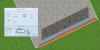
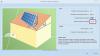
Hello LiamMay, yes this is a known issue. It will be fixed in Version 2017 coming at the end of October. In the meantime you could extrude a "Fireproof Wall" at the edge you are interested in. (see Screenshot1 ) A fireproof wall has an absolute orientation. You could use this value to orientate the module row equally. (see Screenshot2 ). You have to do this accurate and it works.
-
[Transkript] Eine andere Dimension: PV*SOL premium Die neuen Features 2016: (3D-Visualisierung) 1. Bemaßungsplan 2. Vervielfältigen von 3D-Objekten 3. Modulreihen aufziehen 4. Komplexe inkl. Verschaltung kopieren 5. Kartenimport und Extrudieren von 3D-Objekten (Hauptprogramm) 6. Ein- oder zweiachsige Nachführung 7. Netzautarke Systeme in AC-Kopplung 8. Weitere Features Feature 1: Bemaßungsplan Der neuen Button für den Bemaßungsplan befindet sich in der "Modulbelegung" und "Modulaufständerung" Klicken Sie auf diesen Button, um in den Bemaßungsplan zu gelangen. Bemaßt wird die Belegungsfläche, ..ein einzelnes verbautes PV-Modul, ..die Modulabstände innerhalb einer Modulformation ... und der Abstand des ersten Moduls einer Formation zum Giebel und zur Traufe. Klicken Sie auf diesen Button, um den Bemaßungsplan nach *.dxf zu exportieren. Sie können sich diese Datei in einem DXF-Viewer anschauen oder in einem CAD-Programm weiter bearbeiten. Bemaßungspläne sind auch für Flachdächer mit aufgeständerten Anlagen verfügbar. Dies schauen wir uns im nächsten Beispiel an. Hier befindet sich der neue Button in der "Modulaufständerung". Bei den aufgeständerten Anlagen wird zusätzlich der Reihenabstand und die Orientierung der Modulreihen zur Dachkante angezeigt. Der Bemaßungsplan ist an zwei weiteren Orten im Programm abrufbar. Unter Plan/ Bemaßungsplan wird für jede Belegungsfläche ein Bemaßungsplan ausgegeben. Der Plan kann auch dem Projektbericht hinzugefügt werden. Feature 2: "Vervielfältigen von 3D-Objekten" Um in den Dialog "Vervielfachen" zu gelangen, machen Sie einen Rechtsklick auf das entsprechende 3D-Objekt und klicken im Kontextmenü den Menüpunkt "Vervielfachen". Die erzeugten 3D-Objekte werden in einer Formation angeordnet. Geben Sie hierzu die Anzahl Objekte horizontal und vertikal an. .. sowie den Abstand der Objekte zueinander. Klicken Sie anschließend auf "Erzeugen". Mithilfe des "x"-Buttons können die erzeugten Objekte für einen weiteren Versuch wieder entfernt werden. Feature 3: "Das Aufziehen von Modulreihen" Um das Aufziehen zu starten, klicken Sie diesen Button. Wenn Sie mehrere Formationen nacheinander aufziehen möchten, setzen Sie das Häkchen bei "Mehrfach aufziehen". Ziehen Sie nun mit gedrückter linker Maustaste ein Rechteck auf. Im Zentrum des Rahmens wird die Reihenanzahl, sowie die Anzahl PV-Module und die Peak-Leistung ausgegeben. Beim Loslassen werden Sie gefragt, ob Sie die aktuelle Formation ablegen möchten. Um einen neuen Versuch zu starten, klicken Sie "Abbrechen". Wir klicken "OK"! Modulreihen können darüber hinaus mit einem bestimmten Winkel zur Unterkante der Belegungsfläche aufgezogen werden (Im folgenden Beispiel bei -45°). So sieht dann die fertige Reihenformation aus. Feature 4: Kopieren eines gesamten Komplexes mit allen Aufbauten inklusive der Verschaltung. Die vorliegenden PV-Module sind komplett mit Wechselrichtern verschaltet. Um ein 3D-Objekt zu kopieren, machen Sie einen Rechtsklick auf das entsprechende 3D-Objekt und klicken im Kontextmenü den Menüpunkt "Kopieren". Es öffnet sich der Dialog "Zwischenablage". Die Option zum Kopieren der Verschaltung ist bereits angehakt. Ziehen Sie nun mit gedrückter Maustaste eine Kopie des 3D-Objekts aus der Zwischenablage. Die Aufbauten, sowie die gesamte Verschaltung wurden mitkopiert. Natürlich können Sie 3D-Objekte mit allen Aufbauten und der Verschaltung auch mehrfach kopieren. Setzen Sie dazu den Haken bei "Mehrfach kopieren". Feature 5: "Kartenimport und Extrudieren von 3D-Objekten" Dieses Feature wird in einer Vielzahl ausführlicher Video-Tutorials vorgestellt. Siehe: Feature 6: Ein- und zweiachsige Nachführung Klicken Sie im Hauptmenü auf den Button "PV-Module". Im Bereich "Nachführung" können Sie zwischen verschiedenen Nachführsystemen wechseln. System 1: "1-achsig Nord-Süd" Die Module werden Richtung Süden ausgerichtet und es wird eine Drehung um die Nord-Süd-Achse ermöglicht. Die Modulneigung wird über die Neigung der Drehachse festgelegt. Klicken Sie auf diesen Button, wenn Sie die Neigung mithilfe der Klimadaten optimieren möchten. System 2: 1-achsig Ost-West: Die Module werden horizontal mit einer Ausrichtung von 270° montiert. System 3: 1-achsig vertikale Drehachse: Die Module werden mit festem Neigungswinkel aufgeständert und über die Drehung der vertikalen Achse dem Sonnenazimut nachgeführt. System 4: 2-achsig: In diesem Fall wird eine Drehung des Moduls über zwei Achsen ermöglicht. Feature 7: Netzautarke Systeme in AC-Kopplung (SMA Systeme) SMA OffGrid Systeme mit AC-Kopplung Mit oder ohne Dieselgenerator Lastabwurf für Verbrauchergruppen Multi-Cluster möglich 1- und 3-phasige Systeme Hier können Sie die OffGrid-Anlagenart wählen. "Netzautarke PV-Anlage ohne Zusatzgenerator" und "Netzautarke PV-Anlage mit Zusatzgenerator" Wir wählen zuerst die Anlagenart mit Zusatzgenerator. Die Verbraucher können in beliebig vielen Gruppen definiert werden. Für jede Gruppe kann der Lastabwurf eingestellt werden (Uhrzeit und SOC). Hier wird der Dieselgenerator definiert. Sie können die Regelung nach Batterie-Ladezustand.. ..oder nach Verbraucherlast wählen. Hier werden die Batteriewechselrichter und Batterien definiert. Hierfür gibt es auch einen praktischen Auslegungs-Assistenten. Es können beliebig viele Cluster definiert werden. Cluster sind Gruppen von Batterie-Wechselrichtern und Batterien. Im Ergebnis-Überblick sehen Sie die Monatsbilanz der wichtigsten Energien (Verbrauch, PV, Batterien und Diesel). Hier sehen Sie, dass der Verbrauch komplett gedeckt werden konnte. 82,7% des Verbrauchs konnte durch die PV-Anlage versorgt werden. Der Rest musste vom Dieselgenerator übernommen werden. Jetzt wollen wir das gleiche System ohne Dieselgenerator simulieren. Der Verbrauch konnte nun nicht komplett durch die PV-Anlage gedeckt werden, der Lastabwurf wurde aktiv. 3500 kWh wurden ‚abgeworfen‘. Weitere Features Folgenden Features werden vorgestellt: In der Wechselrichterauswahl werden nun auch nicht passende Wechselrichter angezeigt. Einer Verschaltung können nun auch mehrere Anlagen-Wechselrichter über ein Multiplikator zugeordnet werden. PV-Module müssen nur noch einmal ausgewählt werden und können anschließend für alle anderen Modulflächen übernommen werden. In der Wechselrichterauswahl werden nun auch nicht passende Wechselrichter angezeigt. Im Hinweis wird angegeben, warum dieser Wechselrichter nicht passt. Einer Verschaltung können nun auch mehrere Anlagen-Wechselrichter über ein Multiplikator zugeordnet werden. PV-Module müssen von nun an nur noch für eine Modulfläche ausgewählt werden und können anschließend für alle anderen Modulflächen übernommen werden. Ende des Tutorials. Bei dem vorgestellten Programm handelt es sich um PV*SOL premium, eine Planungssoftware der Firma Valentin Software aus dem Bereich Photovoltaik (Regenerative Energien). Schwerpunkte dieser Software sind die Planungsunterstützung und Ertragsprognose. Mit der integrierten 3D-Visualisierung wird der Einfluss der Abschattung auf den Ertrag berücksichtigt. Ein weiterer Schwerpunkt ist die Wirtschaftlichkeit von Photovoltaikanlagen mit und ohne Eigenverbrauch. © 2016 Valentin Software GmbH Stralauer Platz 34 10243 Berlin Germany Tel: +49 (0)30 588 439-0 E-Mail: info@valentin-software.com Weitere Informationen und kostenlose Testversionen: www.valentin-software.com
-
Free trial versions: http://www.valentin-software.com/services/fw/yt-tut-en/dl-pvsolprem-en Software-Tutorial PV*SOL premium (from Version 2016) - Measuring building dimensions with Google Earth Pro - Importing own map sections (tiles?) - Extruding 3D objects This tutorial shows how quickly and easily you can create simple standard buildings and configure a photovoltaic system in PV*SOL premium 2016 without a costly local meeting. In this release, many time-consuming steps have been simplified, considerably accelerating the design process. This is achieved mainly through the new features "Map Import" and "Extrusion Of 3D Objects" Missing dimensions can be measured with Google Earth Pro. High-resolution screenshot of the roof can be made with it too. First, start Google Earth Pro. The installation file and the license key of the software, go to: http://www.google.com/earth/download/gep/agree.html Enter the approximate address of the future location of the PV system and click the button "Search". The software automatically zooms into the vicinity of the site. We are interested in this object. You can move the 3D model with the left mouse button and you can zoom in or out of the map section using the scroll wheel. Alternatively you can use these buttons. Now move the target object to the center of the editor so that you can measure it properly. Click on the button with the ruler icon to open the dialog "Ruler". Now click on the tab "3D path". With this function you can create three-dimensional distance lines to the outer surfaces of the "Auto-Generated Meshes". First, we want to determine the object's height and we focus on a visible line of the complex. Click with the left mouse button on the bottom edge of the object and then on the top edge. The length of the resulting path can be read here. Write down this length. You will need it later. Now bring yourself in a good position to measure out one length of the roof, and make a note of this as well. You will need it later for determining the scale in PV*SOL premium. If there are superstructures on the complex, these can also be measured. Finally, we also need a high resolution screen shot of the complex from the exact bird's eye view. Click on the "N" icon on the navigation menu. For PV*SOL the map section should be facing north. After that, make the screenshot and save it as a file in one of the following formats: *.jpg, *.png or *.bmp. Now start PV*SOL premium 2016 or a later version.You are now on the "Welcome Page" of the application. Please begin a new project and enter your climate data location. Now click on the button "3D Design" and then on the overview screen to get into the "3D Visualization". In the dialog "New 3D System" click on the button "Coverable Object" and select the menu item "Map Section" in the drop down menu. Now you see an expanded view of the dialog. Click on the button with the label "Load From Hard Drive". Load the custom built screenshot from the folder where you have saved it. Now click on the button with the gear icon. It opens the dialog "Determine Scale". Here we have to reproduce the path that we measured in Google Earth. Therefore we re-trace the path between the right and left edges of the building again. Enter the dimension we noted down before in this field. In our example, this results in a scale of 8,42 pixels per meter. The map section is now fully defined. Click on “Start” to begin the project. The software zooms immediately into the "Object View" on the map, and you can begin to sketch the floor plans. At first we sketch a polygon for the target building. Click on this button to begin the process. The polygon can be drawn by clicking on the map section. Please draw accurately. As it may take a while, we will accelerate it. You can interrupt tracing and draw a further polygon with the Enter Key. With the Right Mouse Button or the Escape Key you can terminate the sketching. The plan can then be extruded. Click on the polygon and select the context menu item "Extrude 3D Object". It opens the dialog "Recognize 3D Object". All dimensions as well as the orientation are already taken from this building. And the map section, where the building stands, has already been transferred as texture to the roof surfaces of the flat roof. Enter the measured height in the field "Height". Then click OK. As you can see, we have created a really complex flat roof building PV*SOL offers an automatic method of assigning the modules, which guarantees the optimal utilization of the roof space. So in the next step certain areas of the roof must be blocked. For this, our building must be added to the coverable objects. Then click "Activate". Since the map section was transferred to the roof, other roof structures are now visible, which can also be traced. The end result looks like this. Since mounted PV modules are to be placed on the roof surface, you first have to create and dimension a mounting system. Open the dialog "Edit Assembly System". Here you can specify the "Module Mount", the "Orientation" and "Placing" of the system. We want to place the PV modules horizontally... and two vertical modules. It opens the dialog "Calculate Relative Orientation". Here we enter the desired "Resulting Module Inclination" of 12° and the "Resulting Module Orientation" of 180° (southern exposure). We leave the other default settings unchanged and only want to optimize the orientation. To do this, hit the "Calculate" button. The dialog "Calculate Relative Orientation" then opens. Here we enter the desired "Resulting Module Inclination" of 12° and the “Resulting Module Orientation” of 180° (southern exposure). The program determines the system angles relative to the roof. The system will be mounted later using this information. The mounting system is now adequately dimensioned for our purposes. Click "OK" to create it. Then click this button to perform an optimum coverage of the roof with the module rows. Now you can do a shade frequency calculation to see which PV modules are heavily shaded. End of tutorial Thanks for watching! The computer program featured is PV*SOL premium, a design software from Valentin Software in the fields of photovoltaics and renewable energy. The software focuses on design support and yield calculation. The integrated 3D visualization determines the impact of shading on the yield. PV*SOL premium also calculates the cost-effectiveness of photovoltaic systems with and without self-consumption. Description tags: Type of video: Tutorial, Lesson, Exercise, Practice, Presentation, Demonstration Type of featured software: Google Earth Pro: Geodata Software, Virtual Globe, Map and geographical information program, Relevant Features for PVSOL: 3D Maps, Capability to show 3D buildings and structures, Satellite Images, Address Finder, PV-SOL premium: Photovoltaic Application, Solar Calculator, 3D-Visualization, CAD-Tool, 3D-Sketchup-Tool, Shading Generator, Time-Step Simulation Program, Planning Software, Calculation Program, Spreadsheet Program, Economy Software Features: (Virtual) Photovoltaic System, PV Module, Solar Module, Solar Panel, Solar Cells, PV Array, Free Standing, Rack Mounted Arrays, Inverter, Inverter Configuration, PV Array Configuration, Grid-connected System, Stand-alone PV Systems, Planning, Sizing, Commissioning, System Concept, Inverter Concept, Electricity Consumption, Yield Calculation, Storage, MPP Tracking, 3D-Visualization, Shading Analysis, Shading Animation, Profit Calculation, Profitability Assessment Business Field: Renewable Energy, Sustainable Energy, New Energies, Environmental Engineering, Climate Change, Climate Protection, Decentralized Energy Supply, Solar Energies, Photovoltaics, Power Grid, Market Incentive Program, Solar Market, Customers: PV Planer, Plant Engineers, Craftsmen, Experts, Specialists, Plumbers, Consultants, Installation Firms, Commercial Customers, Manufacturers, System Developers, Universities, Students, Trainees
-
Transskript: Software Tutorial PV*SOL premium Map Import and Extrusion Of 3D Objects (Since Version 2016) This tutorial shows how quickly and easily you can create simple standard buildings and configure a photovoltaic system in PV*SOL premium 2016 without a costly local meeting. In this release, many time-consuming steps have been simplified, considerably accelerating the design process. This is achieved mainly through the new features "Map Import" and "Extrusion Of 3D Objects" First, start PV*SOL premium 2016 or a later version. You are now on the "Welcome Page" of the application. We will now reproduce a simple house with a hipped roof. Please begin a new project. We have chosen Los Angeles as the location. Now click on the button "3D Design" and then on the overview screen to get into the "3D Visualization". In the dialog "New 3D System" click on the button "Coverable Object" and select the menu item "Map Section" in the drop down menu. Now you see an expanded view of the dialog, in which a city map is shown on the top right. Click on it. This opens a new dialog with a large map. The map service that provides the map data is "Bing Maps" from Mircrosoft. This service offers high-resolution aerial photographs, especially in urban areas. An address field is located on the top left, in which you can mark off the location of the building. We are interested in this object. Use the arrow buttons and the buttons with the magnifying glass icon next to the address field to adjust the map section, so that the target building and relevant surrounding shading objects can be seen on it. You can scroll with the mouse wheel and you can move the image with the left mouse button. The resulting "pixels per meter" determined by the map service are shown in the field "scale". If you have different data available, you can change the value. Alternatively, you can also use your own map sections, floor plans or cadastral maps and upload them as image files from the hard disk. Click on "Start" to begin the project. The software zooms immediately into the "Object View" on the map, and you can begin to sketch the floor plans. At first we sketch a polygon for the target building. Click on this button to begin the process. The polygon can be drawn by clicking on the map section. Please draw accurately. You can interrupt tracing and draw a further polygon with the Enter Key. Because the house is a building with a hipped roof, we draw a distance which marks the ridge in the next step. With the Right Mouse Button or the Escape Key you can terminate the sketching. If you have forgotten a corner, you can insert it by pressing the Shift Key + Mouse Click later on. The plan can then be extruded. Click on the polygon and select the context menu item "Extrude 3D Object". It opens the dialog "Recognize 3D Object". Since the ridge is drawn slightly shorter than the longer side of the ground floor, the structure was automatically recognized as "Rectangular 3D Object With Ridge" and a "Building With Hipped Roof" is then offered as the preselection. All dimensions as well as the orientation are already taken from this building. And the map section, where the house stands, has already been transferred to the roof surfaces of the hipped roof. Now only the data for the eaves must be entered, i.e. the height of the ground floor and the roof slope to the longer eave. This data cannot be read out of the map section and should be requested from the end customer. Here we have some shading caused by a tree. This can also be sketched and will be included in the shading simulation. Since the object is to be covered with PV modules in the next step, it must be added to the coverable objects. Then click "Activate". PV-SOL offers an automatic method of assigning the modules, which guarantees the optimal utilization of the roof space. We can execute a shading analysis now. So hit this button. You will see some moderate shading on the bottom right. The PV module is uneconomical and can be removed. End of tutorial Thanks for watching! For more PV*SOL premium tutorials please check out my channel. You can also start discussions on feed-in tariffs, renewable energy, energy policy, funding, etc. The computer program featured is PV*SOL premium, a design software from Valentin Software in the fields of photovoltaics and renewable energy. The software focuses on design support and yield calculation. The integrated 3D visualization determines the impact of shading on the yield. PVSOL premium also calculates the cost-effectiveness of photovoltaic systems with and without self-consumption. Similar to: Google Sketchup


